14.1. Linear Models
14.1.1. Cooked-up Examples
We start with a simple linear model \(y = 2x\). We will generate some test samples containing pairs of (x,y) values. Our goal would be to train a simple linear model \(y = w x\) with the test data and estimate the value of \(w\).
Let us prepare some test data:
> x <- 1:10
> y <- 2*x
Let us fit a model y~x meaning y is linearly dependent on x (with a possible bias term) as
The goal of fitting the model is to compute the weight coefficient w and the intercept or
bias or offset term c:
> lmfit <- lm(y~x)
We can print the model:
> lmfit

Call:
lm(formula = y ~ x)

Coefficients:
(Intercept)            x
  2.247e-15    2.000e+00
The coefficients can be extracted separately:
> coefficients(lmfit)
 (Intercept)            x
2.246933e-15 2.000000e+00
The fitted y values for every value of x:
> fitted.values(lmfit)
 1  2  3  4  5  6  7  8  9 10
 2  4  6  8 10 12 14 16 18 20
This looks too good to be true. Let’s add an intercept term and also introduce some noise:
> n <- length(x)
> e <- rnorm(n, sd = 0.1)
> y <- 2*x + 3 + e
Fitting the linear mode:
> lmfit <- lm(y~x)
> lmfit

Call:
lm(formula = y ~ x)

Coefficients:
(Intercept)            x
      2.933        2.008
The intercept value is very close to 3 and the weight is also pretty close to 2.
Let’s compare the fitted values with actual values of y:
> fitted.values(lmfit)
        1         2         3         4         5         6         7         8         9
 4.941002  6.949160  8.957318 10.965476 12.973634 14.981792 16.989951 18.998109 21.006267
       10
23.014425
> y
 [1]  4.941495  6.895725  9.110955 10.874365 12.980755 14.998704 16.899220 19.066500
 [9] 20.932681 23.076735
We can also see the residual values:
> residuals(lmfit)
            1             2             3             4             5             6
 0.0004929328 -0.0534350207  0.1536365592 -0.0911108850  0.0071203406  0.0169111935
            7             8             9            10
-0.0907301344  0.0683915230 -0.0735859540  0.0623094450
Let’s look at more complicated models.
A polynomial in x:
> y <- 3 + 4*x + 5 *x^2 + rnorm(n, sd=0.1)
> lmfit <- lm(y~1+x+I(x^2))
> lmfit

Call:
lm(formula = y ~ 1 + x + I(x^2))

Coefficients:
(Intercept)            x       I(x^2)
      2.945        3.965        5.005
Multiple sinusoidal variables:
> x <- sin(pi *seq(0, 2, by=0.05))
> y <- cos(pi *seq(0, 2, by=0.05))
> n <- length(x)
> z <- 2 + 3*x + 4*y + rnorm(n, sd=0.1)
> lmfit <- lm(z~x+y)
> lmfit

Call:
lm(formula = z ~ x + y)

Coefficients:
(Intercept)            x            y
      2.014        2.982        4.015
With just 41 samples, the estimate is pretty good.
Fitting without the intercept term:
> z <- 2 + 3*x + 4*y + rnorm(n, sd=0.1)
> lm(z~0+x+y)

Call:
lm(formula = z ~ 0 + x + y)

Coefficients:
    x      y
2.982  4.111
We note that the original formula had an intercept term. This had an undesired effect on the estimate of the weights of x and y.
Let us consider an example where the construction of z doesn’t have an intercept term:
> z <- 3*x + 4*y + rnorm(n, sd=0.1)
> lmfit <- lm(z~0+x+y)
> lmfit

Call:
lm(formula = z ~ 0 + x + y)

Coefficients:
    x      y
3.003  3.984
> coefficients(lmfit)
       x        y
3.003388 3.983586
We see that the weights of x and y are calculated correctly.
Fitting on a data frame
Let’s explore the relationship between the mpg and disp variables in the mtcars dataset.
Attaching the dataset:
> attach(mtcars)
Exploring a polynomial dependency:
> lmfit <- lm(disp~1+mpg+I(mpg^2))
> lmfit

Call:
lm(formula = disp ~ 1 + mpg + I(mpg^2))

Coefficients:
(Intercept)          mpg     I(mpg^2)
   941.2143     -53.0598       0.8101
Measuring the quality of estimation as ratio between residuals and fitted values:
> mean(abs(residuals(lmfit) / fitted.values(lmfit) ))
[1] 0.1825118
14.1.2. Cars Data Set
cars dataset is shipped with R distribution. It captures the speed of
cars vs the distance taken to stop the car. This data was recorded in 1920s.
The data set consists of 50 records:
> dim(cars)
[1] 50  2
Summary statistics:
> summary(cars)
     speed           dist
 Min.   : 4.0   Min.   :  2.00
 1st Qu.:12.0   1st Qu.: 26.00
 Median :15.0   Median : 36.00
 Mean   :15.4   Mean   : 42.98
 3rd Qu.:19.0   3rd Qu.: 56.00
 Max.   :25.0   Max.   :120.00
Let us create a scatter plot of speed vs distance data:
> qplot(speed, dist, data=cars)
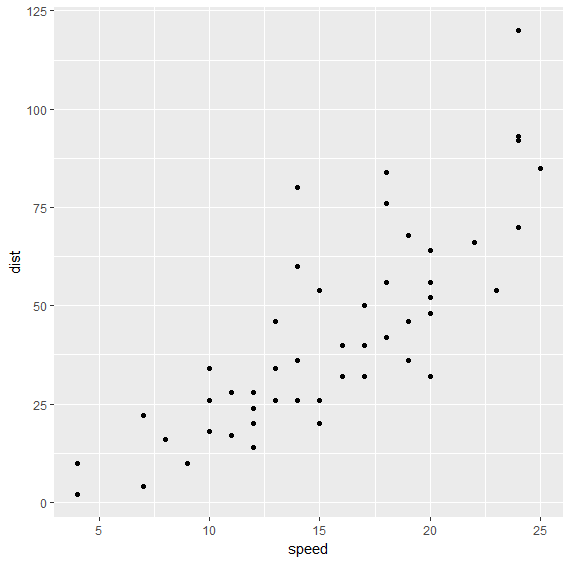
There appears to be a good correlation between speed and distance and the relationship appears to be quite linear. Let us verify the correlation between the two variables too:
> cor(cars)
          speed      dist
speed 1.0000000 0.8068949
dist  0.8068949 1.0000000
Let us fit a linear model dist = a + b speed to this dataset:
> fit <- lm(dist~speed, data=cars)
> fit

Call:
lm(formula = dist ~ speed, data = cars)

Coefficients:
(Intercept)        speed
    -17.579        3.932
The fitted values for distance are:
> round(fitted.values(fit), 2)
    1     2     3     4     5     6     7     8     9    10    11    12    13    14    15    16    17    18    19
-1.85 -1.85  9.95  9.95 13.88 17.81 21.74 21.74 21.74 25.68 25.68 29.61 29.61 29.61 29.61 33.54 33.54 33.54 33.54
   20    21    22    23    24    25    26    27    28    29    30    31    32    33    34    35    36    37    38
37.47 37.47 37.47 37.47 41.41 41.41 41.41 45.34 45.34 49.27 49.27 49.27 53.20 53.20 53.20 53.20 57.14 57.14 57.14
   39    40    41    42    43    44    45    46    47    48    49    50
61.07 61.07 61.07 61.07 61.07 68.93 72.87 76.80 76.80 76.80 76.80 80.73
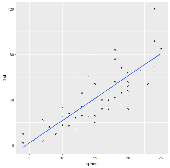
We can plot the fitted values as follows:
> ggplot(data=cars, mapping=aes(x=speed, y=dist)) + geom_point(shape=1) + geom_smooth(method='lm', se=FALSE)
14.1.2.1. Diagnostics
We can print the summary statistics for the linear model as follows:
> fit.summary <- summary(fit); fit.summary

Call:
lm(formula = dist ~ speed, data = cars)

Residuals:
    Min      1Q  Median      3Q     Max
-29.069  -9.525  -2.272   9.215  43.201

Coefficients:
            Estimate Std. Error t value Pr(>|t|)
(Intercept) -17.5791     6.7584  -2.601   0.0123 *
speed         3.9324     0.4155   9.464 1.49e-12 ***
---
Signif. codes:  0 ‘***’ 0.001 ‘**’ 0.01 ‘*’ 0.05 ‘.’ 0.1 ‘ ’ 1

Residual standard error: 15.38 on 48 degrees of freedom
Multiple R-squared:  0.6511,    Adjusted R-squared:  0.6438
F-statistic: 89.57 on 1 and 48 DF,  p-value: 1.49e-12
Several important statistics can be separated out.
R Squared:
> fit.summary$r.squared
[1] 0.6510794
Adjusted R Squared:
> fit.summary$adj.r.squared
[1] 0.6438102
F Statistic:
> fit.summary$fstatistic
   value    numdf    dendf
89.56711  1.00000 48.00000
The ggfortify library provides functions to let ggplot interpret linear models:
> install.packages("ggfortify")
> library(ggfortify)
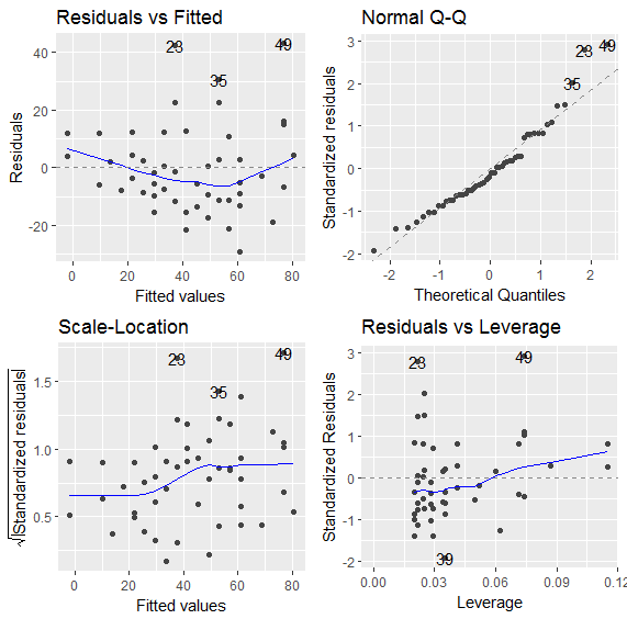
We are now ready to plot the diagnostics for this model:
> autoplot(fit)
14.1.3. Cats Data Set
This data set is available in MASS package. The data set records body weight and heart weight for 144 cats along with their sex.
Loading the dataset:
> data(cats, package='MASS')
Variables in the data set:
> str(cats)
'data.frame':   144 obs. of  3 variables:
 $ Sex: Factor w/ 2 levels "F","M": 1 1 1 1 1 1 1 1 1 1 ...
 $ Bwt: num  2 2 2 2.1 2.1 2.1 2.1 2.1 2.1 2.1 ...
 $ Hwt: num  7 7.4 9.5 7.2 7.3 7.6 8.1 8.2 8.3 8.5 ...
Few rows from data set:
> head(cats)
  Sex Bwt Hwt
1   F 2.0 7.0
2   F 2.0 7.4
3   F 2.0 9.5
4   F 2.1 7.2
5   F 2.1 7.3
6   F 2.1 7.6
Summary statistics:
> summary(cats)
 Sex         Bwt             Hwt
 F:47   Min.   :2.000   Min.   : 6.30
 M:97   1st Qu.:2.300   1st Qu.: 8.95
        Median :2.700   Median :10.10
        Mean   :2.724   Mean   :10.63
        3rd Qu.:3.025   3rd Qu.:12.12
        Max.   :3.900   Max.   :20.50
Predicting the heart weight from body weight:
> fit <- lm(Hwt~Bwt, data=cats)
> fit

Call:
lm(formula = Hwt ~ Bwt, data = cats)

Coefficients:
(Intercept)          Bwt
    -0.3567       4.0341
Summary statistics for the fitted model:
> summary(fit)

Call:
lm(formula = Hwt ~ Bwt, data = cats)

Residuals:
    Min      1Q  Median      3Q     Max
-3.5694 -0.9634 -0.0921  1.0426  5.1238

Coefficients:
            Estimate Std. Error t value Pr(>|t|)
(Intercept)  -0.3567     0.6923  -0.515    0.607
Bwt           4.0341     0.2503  16.119   <2e-16 ***
---
Signif. codes:  0 ‘***’ 0.001 ‘**’ 0.01 ‘*’ 0.05 ‘.’ 0.1 ‘ ’ 1

Residual standard error: 1.452 on 142 degrees of freedom
Multiple R-squared:  0.6466,    Adjusted R-squared:  0.6441
F-statistic: 259.8 on 1 and 142 DF,  p-value: < 2.2e-16
The t-value for intercept term is small. This is indicative that if body weight is 0, then heart weight will also be 0.
Let us check if including the sex of the cat provides any help in improving the model:
> fit2 <- lm(Hwt~Bwt+Sex, data=cats)
> fit2

Call:
lm(formula = Hwt ~ Bwt + Sex, data = cats)

Coefficients:
(Intercept)          Bwt         SexM
    -0.4150       4.0758      -0.0821

> summary(fit2)

Call:
lm(formula = Hwt ~ Bwt + Sex, data = cats)

Residuals:
    Min      1Q  Median      3Q     Max
-3.5833 -0.9700 -0.0948  1.0432  5.1016

Coefficients:
            Estimate Std. Error t value Pr(>|t|)
(Intercept)  -0.4149     0.7273  -0.571    0.569
Bwt           4.0758     0.2948  13.826   <2e-16 ***
SexM         -0.0821     0.3040  -0.270    0.788
---
Signif. codes:  0 ‘***’ 0.001 ‘**’ 0.01 ‘*’ 0.05 ‘.’ 0.1 ‘ ’ 1

Residual standard error: 1.457 on 141 degrees of freedom
Multiple R-squared:  0.6468,    Adjusted R-squared:  0.6418
F-statistic: 129.1 on 2 and 141 DF,  p-value: < 2.2e-16
We note that the residual standard error has increased and the F statistic has decreased. We see that t-value for the sex parameter is very small. It doesn’t add value to the model.